Reinforcement learning, lesson 1

Introduction

Basic RL model

In any RL model, there is :

an RL agent
an Environment, deterministic or stochastic
actions
rewards ( long/short term, intermediate)
states (known/unknown)
a goal: maximizing the reward function

RL is a Framework for learning by interaction under uncertainty. An agent takes actions, receives rewards, and the environment evolves to the next state.

1. Markov Decision Process

A RL problem is modelled using Markov Decision Processes.

The RL interactions

The classic RL interaction is as follows:

We have a discrete decision time $t$ (which would be for example seconds), and at each timestamp :

The agent selects an action $a_t$, based on $s_t$ the current state of the system.
The agent gets his reward $r_t$
The Environment moves to a new state $s_{t+1}$

📝 Markov chains

Markov Chains are the building blocks of RL. A Markov Chain is a stochastic (which means that it includes randomness ) model describing a sequence of possible events in which the probability of each event depends only on the state attained in the previous event¹. In order to create a model, we need to introduce mathematical definitions.

Definition : Given $S$, a state space and a bounded compact subset of the Euclidean space, the discrete time dynamic system $(s_t)_{t\in \mathbb{N}}$ is a markov Chain if it satisfies the Markov property:

$$ \mathbb{P}\left(s_{t+1}=s \mid s_{t}, s_{t-1}, \ldots, s_{0}\right)=\mathbb{P}\left(s_{t+1}=s \mid s_{t}\right)$$

📝 Markov Decision Process (MDP)

A Markov Decision Process is a tool, to model decision making when outcomes can be random.

Definition : a Markov Decision Process is defined as a tuple $M=(S,A,p,r)$ with

$S$ the (finite) State space

$A$ the (finite) Action space

$p(s'|s,a)$ the transition probability, such that $\mathbb{P}\left(s_{t+1}=s' \mid s_{t}=s,a_t=a\right)$

$r(s,a,s')$ is the reward of the transition from $s$ to $s'$ taking the action $a$. The reward can be stochastic, but we can express its distribution, $v$ for $s,a$ as $v(s,a)$. Thus the reward can be writtent as : $r(s,a) = \mathbb{E}_{R\sim v(s,a)}[R]$.

Assumptions

Markov assumptions : the current state $s$ and the action $a$ are a sufficient statistic for the next state $s'$. This means that “no other statistic that can be calculated from the same sample provides any additional information as to the value of the parameter”². Our statistic provides as much information as possible.

Time assumption : discrete time, at each step, $t\leftarrow t+1$.

Reward assumption : the reward is uniquely defined by a transition from a state $s$, to $s'$ and an action $a$.

Stationary assumption : transition and reward don’t change with time. Otherwise, it’s non-stationary.

2. Policy

Definition : a decision rule $d$, which chooses an action from the state $S$ of the system can be :

Deterministic, given the same set of state $S$, the action $a\in A$ will be chosen

Stochastic, a probability distribution over the actions determines $a$.

Then, it can also be :

( stochastic / deterministic ) History-dependant

( stochastic / deterministic ) Markov (relies on the previous state)

Definition : A policy is a sequence of decision rules, it can be :

Non-stationary, then $\pi = (d_0,d_1,…)$

stationary, then $\pi = (d,d,…)$

At each round t, an agent following the policy $\pi$ selects the actions $a_t \sim d_t(s_t)$ .

Markov chain of a policy

The transition probability of a random process $(s_t)_{t \in \mathbb{N}}$ with regards to a stationary policy $\pi$ is the following :

$$ p^\pi (s'\mid s) = \mathbb{P}(s_{t+1}=s' \mid s_t = s, \pi) $$

Every actions in $A$ (even if it does not take the state from $s$ to $s'$) has to be taken into account. Thus we deduce that $$ p^\pi (s'\mid s) = \sum_{a\in A} \pi(s,a)p(s'\mid s,a) $$

3. Optimality Principle

How do we evaluate a policy ?

📝 State value function

The state value function allows us to determine the effectiveness of a policy. Various definitions can be used depending on the problem at hand. For the following definitions, let $\pi = (d_1, d_2, …,)$ be a deterministic policy.

🎲 The Finite time horizon T policy, sets a deadline $T$, at which the sum of the rewards up to $T$ will be computed. The value function can be expressed as :

$$ V^\pi(t,s) = \mathbb{E}\left[ \sum_{\tau = t}^{T-1} r(s_\tau,d_\tau(h_\tau)) + R(s_T) \mid s_t = s; \pi = (d_1, d_2, …,) \right ]$$

Here, where $R$ is a value function for the final state. Here we compute the expectation of the sum of the rewards obtained taking actions according to the policy, and receiving the corresponding rewards. We have to take into account the Expectation because the decision process can be stochastic, and thus the Expectation gives the equivalent of the mean rewards in a stochastic model.
$\qquad$📝 It is usually used when there is a deadline to meet.

🎲 The Infinite Time Horizon with discount translates a problem that never terminates. Rewards closer in time receive a higher importance :

$$ V^{\pi}\left(s\right)\ =\ \mathbb{E}\left[\sum_{t=0}^{\infty}\gamma^tr\left(s_t,d_t\left(h_t\right)\right)\ \mid s_{0\ }=s;\pi \right] $$

where $0\leq\gamma<1$ is the discount factor.
$\qquad$📝 We implement it when there is uncertainty about the deadline, or intrinsic definition of discount

🎲 The Stochastic shortest path , the problem never terminates but the agent will reach a termination state.

$$V^{\pi}\left(s\right)\ =\ \mathbb{E}\left[\sum_{t=0}^{T_{\pi}}r\left(s_t,d_t\left(h_t\right)\right)\ \mid s_{0\ }=s;\pi\right]$$

$T_{\pi}$ : first random time when the termination state is achieved.
$\qquad$📝 Used when there is a specific goal condition

🎲 The Infinite time horizon with average reward, the problem never terminates but the agent focuses on the expected average of the rewards

$$V^{\pi}\left(s\right)\ =\ \lim_{T\to\infty}\ \mathbb{E}\left[\frac{1}{T}\sum_{t=0}^{T-1}r\left(s_t,d_t\left(h_t\right)\right)\ \mid s_{0\ }=s;\pi\right]$$

$T_{\pi}$ : first random time when the termination state is achieved.
$\qquad$📝 Used when the system should be constantly controlled over tim

Optimization problem :

Definition : The solution to an MDP is an optimal policy $\pi^$ satisfying $\pi^ \in \underset{\pi \in \Pi}{\text{argmax }} V^\pi$

The value function under that policy is the optimal value function : $V^* = V^{\pi^*}$

🎮 Application :

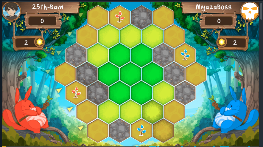
I will use a concrete and fun example of a game, where an RL agent can learn to win. The agent will play the 2021 Coding Game Spring Challenge, the Photosynthesis game (but a bit simplified)

Here, the environment is the board game. Let’s define the various notions that we introduced before in this framework.

🎯 The goal is to end the game with more points than your opponent. For now, let's just say that the goal is to gain as much sun ☀️ as possible.

🌳 The environment in which the game takes place is a forest.

💭 The actions available to the agent are the following :

SEED : Planting a seed. It can only be done in the range of the size of the tree.
GROW : Growing a tree. From a seed (size 0) to a sprout (size 1) to a sapling (size 2) to a mature tree (size 3)
CUT : Cut a tree. Only mature trees can be cut
WAIT : Do nothing

💰 Each action has a reward associated:

Planting a seed costs 1 sun plus number of seeds already on the board-suns. (for example, in the figure above, planting a seed would cost 3 suns)
Growing a tree cost size_of_the_tree-suns plus number of trees withe the same size on the board-suns.
Cutting a tree gives a reward of 3 suns. (let’s forget for now the quality of the soil)
Do nothing

📍 The game state is defined by the current state of the board.

Arthur Zucker